PSTAT100 - Simple linear regression

From last time

statistical models are probabilistic represenations of data generating processes
- some randomness must be present (usually from sampling) for this to be sensible
regression models relate a variable of interest to one or more other ‘explanatory’ variables and consist of:
- a distribution for the variable of interest
- expression(s) for the distribution’s parameters in terms of the explanatory variable(s)
for linear regression, the mean of the response is a linear function of the explanatory variable(s)
- ‘simple’ if one explanatory variable
- ‘multiple’ if many explanatory variables
- ‘multivariate’ if many variables of interest

From last time

A simple linear model is where are ‘residuals’ – leftover quantities.

The least squares line minimizes the sum of squared residuals – i.e., the residual variance, assuming the line passes through the mean.

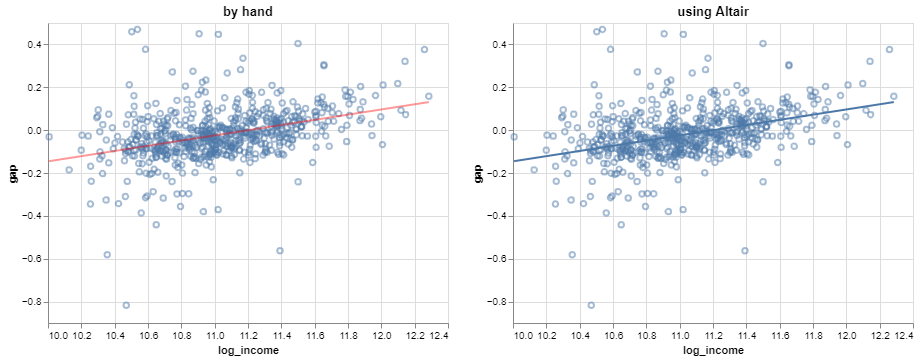
Visualizing the line

Verifying that the line plotted on a prediction grid (left) matches the regression transform from Altair (right):

Not a statistical model, yet

The least squares line is simply an algebraic transformation of the data – technically, a projection.

This is not yet a statistical model according to our definition, since there is no probability distribution involved.

We can change that by considering the residuals to be random.

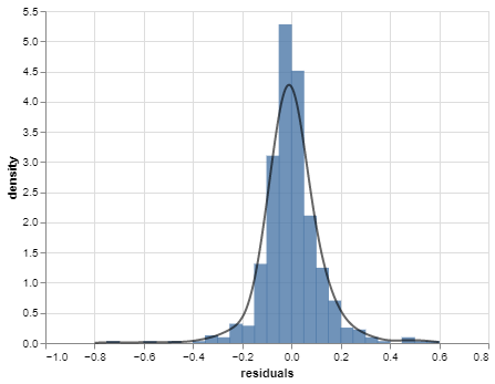
Residual distribution

Have a look at the histogram of the residuals (with a KDE curve):

Does this look like any probability density function you encountered in 120A?

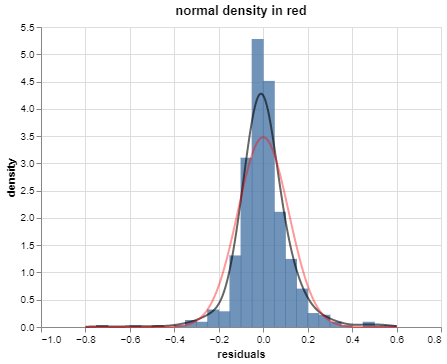
Residual distribution

The residual distribution is pretty well-approximated by the normal or Gaussian distribution:

The error model

This phenomenon – nearly normal residuals – is pretty common in practice.

So a standard distributional model for the residuals is that they are independent normal random variables. This is written as:

This is an important modification because it induces a probability distribution on .

The simple linear regression model

Now we’re in a position to state the simple linear regression model:

is the response variable
is the explanatory variable
is the random error
are the model parameters
- is the intercept
- is the coefficient
- is the error variance

Properties of the normal distribution

As a refresher from 120A, if then:

(Mean)
(Variance)
(Linearity) For constants ,

Model implications

Treating the error term as random has a number of implications that follow from the properties of the normal distribution:

(Normality) The response is a normal random variable:
(Linearity) The mean response is linear in :
(Constant variance) The response has variance:
(Independence) The observations are independent (because the errors are):

These are the assumptions of the simple linear regression model.

Aside: other error distributions, or conditions that don’t assume a specific distribution, are possible.

Estimates

You’ve already seen how to compute the least squares estimates of – these are no different when the errors are random.

Estimates are typically denoted by the corresponding paramater with a hat:

An estimate of the error variance is:

Estimates (matrix form)

These estimates can be expressed in matrix form as:

Fitted values and residuals

The projections of the data points onto the line are the estimated values of the response variable for each data point.

These are known as fitted values and denoted :

Then, the differences between observed and fitted values give the model residuals:

Computations

# retrieve data
x = sm.tools.add_constant(regdata.log_income.values)
y = regdata.gap.values

# fit regression model
slr = sm.OLS(endog = y, exog = x)

# estimates
beta_hat = slr.fit().params

# fitted values
fitted = slr.fit().fittedvalues

# residuals
resids = slr.fit().resid

# error variance estimate
sigmasq_hat = slr.fit().scale

print('coefficient estimates: ', beta_hat)
print('error variance estimate: ', sigmasq_hat)

coefficient estimates:  [-1.35616996  0.12105696]
error variance estimate:  0.01317117061613733

Parameter interpretations: intercept

The intercept represents the mean response when .

In the SEDA example:

For districts with a log median income of 0, the mean achievement gap between boys and girls is estimated to be -1.356 standard deviations from the national average.

Not incorrect, but awkward:

log median income is not a natural quantity
the sign is confusing

Parameter interpretations: intercept

Better:

For school districts with a median income of 1 dollar, the mean achievement gap is estimated to favor girls by 1.356 standard deviations from the national average.

Check your understanding:
- why 1 dollar and not 0 dollars?
- why not -1.356?
Not of particular interest here because no districts have a median income of 1 USD.

Parameter interpretations: slope

The slope represents the change in mean response per unit change in .

In the SEDA example:

Each increase of log median income by 1 is associated with an estimated increase in mean achievement gap of 0.121 standard deviations from the national average in favor of boys.

Not incorrect, but a bit awkward – how much is a change in log median income of 1 unit?

Parameter interpretations: slope

Better:

Every doubling of median income is associated with an estimated increase in the mean achievement gap of 0.084 standard deviations from the national average in favor of boys.

Why doubling??
Hint:

Parameter interpretations: error variance

The error variance represents the variability in the response after accounting for the explanatory variable .

In the SEDA example:

After adjusting for log median income, the gender achievement gap varies among districts by an estimated 0.11 standard deviations from the national average.

Note that is reported for interpretation on the original scale, rather than .

Parameter interpretations: error variance

Compare the estimated ‘raw’ variance in gender gap with the estimated residual variance after accounting for log median income:

Code

print('raw variance: ', y.var(ddof = 1))
print('estimated residual variance: ', sigmasq_hat)

raw variance:  0.015355417268162816
estimated residual variance:  0.01317117061613733

The estimated variability in achievement gap diminishes a little after adjusting for log median income. The relative reduction is:

In the SEDA example, the reduction was about 14%:

Code

print('relative reduction in variance: ',
    (y.var(ddof = 1) - sigmasq_hat)/y.var(ddof = 1)
)

relative reduction in variance:  0.1422459978703541

Parameter interpretations: variance

A closely related quantity is the R-squared statistic, which simply adjusts the denominator of the error variance estimate:

used as a measure of fit
interpreted as the proportion of variation in the response explained by the model

General parameter interpretations

There is some general language for interpreting the parameter estimates:

(Intercept) When [] the mean [response variable] is estimated to be [ units].
(Slope) Every [one-unit increase in ] is associated with an estimated change in mean [response variable] of [ units].
(Error variance) After adjusting for [explanatory variable], the remaining variability in [response variable] is an estimated [ units] about the mean.

You can use this standard language as a formulaic template for interpreting estimated parameters.

Centering the explanatory variable

If we want the intercept to be meaningful, we could center the explanatory variable and instead fit:

Code

# center log median income
log_income_ctr = (regdata.log_income - regdata.log_income.mean()).values

# form x matrix
x_ctr = sm.tools.add_constant(log_income_ctr)

# refit model
slr_ctr = sm.OLS(endog = y, exog = x_ctr)
beta_hat_ctr = slr_ctr.fit().params

# display parameter estimates
print('coefficient estimates: ', beta_hat_ctr)
print('error variance estimate: ', slr_ctr.fit().scale)

coefficient estimates:  [-0.02105724  0.12105696]
error variance estimate:  0.01317117061613733

For a district with average log median income, the estimated achievement gap favors boys by 0.021 standard deviations from the national average.

note that this is just a location shift so other estimates are unchanged
can recover the original intercept estimate as

beta_hat_ctr[0] - beta_hat_ctr[1]*regdata.log_income.mean()

-1.3561699570330035

Other transformations

We could seek to adjust the model so that the intercept is interpreted as the gap at the district with the smallest median income:

But this changes the meaning of the other model terms:

represents the change in mean gap associated with multiplicative changes in the amount by which a district’s median income exceeds that of the poorest district
is the variability of the gap after adjusting for the log of the difference in median income from the median income of the poorest district

Other transformations

Unsurprisingly, estimates are not invariant under arbitrary transformations, so if the meanings of the other parameters change, then so do the estimates:

# center log median income
income = np.exp(regdata.log_income) 
income_shifted = income - income.min()
log_income_shifted = np.log(income_shifted + 1)

# form x matrix
x_shifted = sm.tools.add_constant(log_income_shifted)

# refit model
slr_shifted = sm.OLS(endog = y, exog = x_shifted)
beta_hat_shifted = slr_shifted.fit().params

# display parameter estimates
print('coefficient estimates: ', beta_hat_shifted)
print('error variance estimate: ', slr_shifted.fit().scale)

coefficient estimates:  const        -0.544166
log_income    0.049851
dtype: float64
error variance estimate:  0.01390497936420638

Note also it’s not possible to express the old parameters as functions of the new parameters; this is a fundamentally different model.

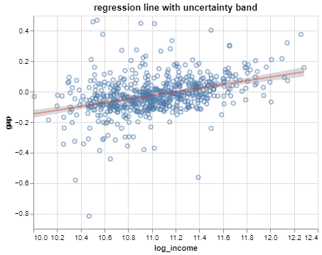
Uncertainty quantification

A great benefit of the simple linear regression model relative to a best-fit line is that the error variance estimate allows for uncertainty quantification.

What that means is that one can describe precisely:

variation in the estimates (i.e., estimated model reliability);
variation in predictions made using the estimated model (i.e., predictive reliability).

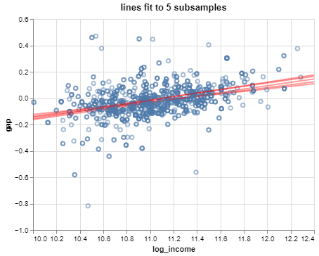
Understanding variation in estimates

What would happen to the estimates if they were computed from a different sample?

We can explore this idea a little by calculating least squares estimates from several distinct subsamples of the dataset.

The lines are pretty similar, but they change a bit from subsample to subsample.

Variance of least squares

How much should one expect the estimates to change depending on the data they are fit to?

It can be shown that the variances and covariance of the estimates are:

Bear in mind that the randomness comes from the model term.

these quantify how much the parameters vary across collections of ’s measured at exactly the same values of
these are not variances of the parameters; and are constants, i.e., not random
they are also not variances of the estimates – e.g., is yet another constant

Standard errors

So the variances can be estimated by plugging in for in the variance-covariance matrix from the previous slide.

The estimated standard deviations are known as standard errors:

Computations and intepretations

The estimated variance-covariance of the least squares estimates is computed by the .cov_params() method:

slr.fit().cov_params()

array([[ 0.01708179, -0.00154692],
       [-0.00154692,  0.00014026]])

the intercept estimate varies by an estimated across datasets, with fixed
the slope estimate varies by an estimated across datasets, with fixed

Confidence intervals

About 95% of the time, the true values will be within 2SE of any particular estimates .

The intervals provide ranges of possible values for the true values :

slr.fit().conf_int()

array([[-1.61283063, -1.09950928],
       [ 0.09779946,  0.14431446]])

This supports two important inferences:

with 95% confidence, the intercept is estimated to be between -1.613 and -1.010
with 95% confidence, the slope is estimated to be between 0.098 and 0.144

And the width of those intervals conveys a sense of the uncertainty associated with the estimates.

Visualizing uncertainty

It’s fairly common practice to add a band around the plotted line to indicate estimated variability.

represents the uncertainty/variability of the parameter estimates, i.e., of the trend line
does not represent the uncertainty/variability of the observations – note the spread of data is considerably broader than the uncertainty band